
Excel spreadsheets are an important tool for analysing data and organising information in the business world.
However, without proper formatting, Excel sheets can become cluttered and difficult to navigate. Proper formatting not only makes your spreadsheets easier to read and use but can also help you avoid errors and ensures consistency in your data presentation.
In this blog post, we will cover some best practices for formatting spreadsheets for business to make your data as clear and usable as possible.
General Best Practises for Formatting Excel Sheets
When setting up a new Excel spreadsheet, it helps to start with some general formatting guidelines. First, make sure to give your sheet a clear and descriptive title by double clicking the existing Sheet1, Sheet2, etc. name that Microsoft Excel provides by default.
Next, add column headers to give your data context. Simply click into the top row of your sheet and input your column names, like “Date,” “Region,” “Sales Amount,” etc. Format these column headers to stand out by making them bold or increasing the font size. You can also right align numeric column headers for easy scanning.
Adjust column widths to avoid truncating data or having excessive white space. Click and drag the right border of the column header to auto-fit the width based on the content. Avoid having columns that are too wide or too narrow for the data range.
Lastly, freeze the top row (your header row) so it remains visible when scrolling down the sheet. To do this, navigate to the View tab and check the Freeze Top Row box.
Using Document Themes for Consistent Branding
Applying document themes allows you to quickly format your whole Excel workbook to ensure it aligns with your company’s branding.
Themes apply colours, fonts, and effects consistently across all sheets, so you don’t need to manually change these each time you create a new Excel document.
To create a custom theme that matches your branding:
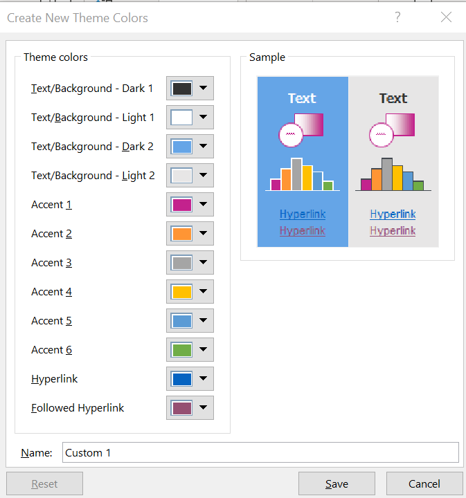
- Go to the Page Layout tab and click on Themes. Choose “Create New Theme”
- In the Theme Colours section, click each dropdown and choose the exact colours for text/background, hyperlinks, followed hyperlinks etc.
- For Theme Fonts, choose the fonts you want applied to Headings and Body text. Make sure to pick fonts which are installed on all users’ systems.
- Finally, for Theme Effects, adjust accent colours used in things like pivot tables or conditional formatting. Tone down these effects if needed.
- Click Save, and finally give your theme a descriptive name.
Now when you want to apply this theme for brand consistency in a new document:
- Go to Page Layout > Themes
- Click the dropdown and select your custom theme under “Custom”
- Click Apply to apply the theme formatting to the entire workbook
Take a look at our Introduction to Excel Course
Using Styles to Format Tables and Charts
Excel styles allow you to apply professional formatting to tables, charts, pivot tables, and other objects with just a few clicks. Styles are preset designs that automatically change colours, fonts, effects, and layouts.
There are several style galleries built into Excel, including:
- Table Styles – Used to format a data table. When you select your data range and click Format as Table on the Home tab, the Table Style gallery appears. It contains many colour and layout choices to instantly convert a plain data range into a stylish, formatted table.
- PivotTable Styles – These styles automatically format your pivot tables with colour variations and layouts. Just insert a pivot table, then apply a style from the PivotTable Styles gallery on the Design tab.
- Chart Styles – Make your charts look polished by applying a Chart Style after insertion. The Styles gallery on the Design tab offers colour palettes and effects to match your document theme.
- Cell Styles – Use these to format individual cells with colours, fonts, and numbering formats that coordinate across your workbook.
Styles save a huge amount of time compared to manually formatting each object. They also allow consistency through uniform colours and fonts. Simply select your table, chart, etc. then browse the style gallery on the appropriate tab to find a look that aligns with your branding. Apply the style with one click for professional instant formatting.
Changing the Orientation of Labels and Headings
For long text strings, change the orientation of column headers from horizontal to diagonal to save space. Simply select the cells, go to the Home tab, and click the Orientation button. Choose an angle between 45 to 90 degrees to best fit the header text.
You can also rotate row labels vertically, so the text reads top to bottom instead of left to right. This can be useful when your space for headings is extremely limited. Right click the row number to access the orientation options. Rotate the text 90 degrees to save horizontal space when you have long row labels.
Using Colours for Readability and Emphasis
Use colour strategically in your Excel sheets to draw attention to important trends or data points, as well as making it easier to read.
For example, you could highlight key metrics like totals and averages in a contrasting color, or always use a specific colour for cells which are calculating a value from other cells.
Techniques such as using alternate row colours can also make scanning tabular data easier on the eyes. Just be sure colours meet accessibility standards for text/background colour contrast.
You can also colour code data by status, like green for on track, yellow for at risk, and red for late. This allows viewers to instantly identify outliers or issues. However, make sure to keep your colour choices limited to avoid overwhelming the spreadsheet.
Using Borders to Segment Data
You have the option to add borders to define sections of your spreadsheet and delineate different types of data.
For instance, you might put a thick bottom border below your headers, or add borders around summarised data to separate from the detailed data rows.
To add a border, select the target cells, then on the Home tab choose a border style and colour that suits your theme. Adjust which sides have borders as needed.
Using Welcome Sheets
Especially if the workbook is intended to be shared externally or with new hires, consider adding a dedicated Welcome or Instructions sheet. This should outline the purpose, structure, definitions, and sources of your spreadsheets.
Make it the first visible sheet on your bar tab so it opens automatically. Use large, friendly fonts and add images if beneficial. You can also link it to key sheets or cells within the workbook to aid navigation.
A welcome page improves usability and can explain guidelines for using or editing the sheets to ensure the right formulas and formatting are preserved.
Getting Started with Conditional Formatting
Conditional formatting allows you to automatically highlight cells that meet criteria you specify, helping identify trends and outliers. For example, you could conditionally format sales numbers red if they fall below a set target amount.
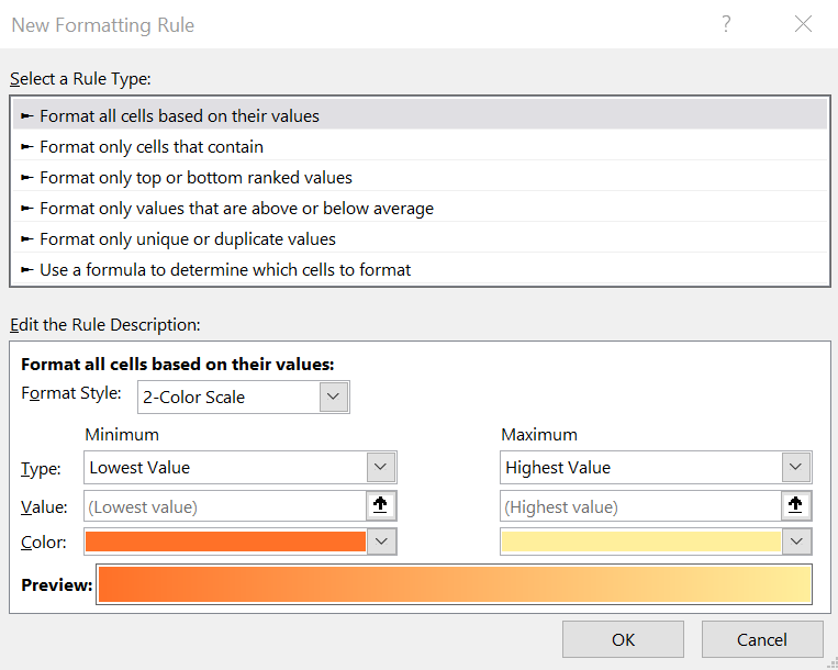
To add a basic conditional format, select your target cells, go to Home > Conditional Formatting, and choose a format like Colour Scales or Data Bars. More options will appear to customise the formatting rule and style.
You can apply multiple conditional formatting rules to highlight different types of important data. Just be careful not to overuse it as too many colours and icons can reduce readability.
Controlling Data Input
It’s often a good idea to control data entry to prevent errors and inconsistencies in your Excel sheet.
It’s possible to limit cell entries to a certain type, like numbers or dates only. You can alternatively restrict choices by creating drop down lists instead of free text fields.
To add a drop down list, select the target cell(s) and go to Data > Data Validation. Choose List from the Allow field, and then input your selections either manually or by cell range reference.
This prevents incorrect or ambiguous data from being entered by users, saving time catching errors in the future.
Conclusion
By mastering spreadsheet formatting techniques, you will save time, avoid errors, and present compelling data insights to stakeholders. With some upfront planning and design work, your Excel sheets can become highly effective decision-making tools for your business.
For structured Excel training tailored to the needs of office professionals, consider the wide range of Microsoft Excel courses available from Elliot Training. Their interactive online and in-person classes can take your Excel skills to the next level.