5 Things you didn’t know about Excel

Microsoft Excel is a crucial tool for a lot of people, helping them with calculations or working with large amounts of data. But have you ever wondered if there are any secret features to Microsoft Excel?

From adding shortcuts to quicken ways to process large amounts of data, here are 5 things you didn’t know about Excel.

Adding Shortcuts Above Your Toolbar

This feature allows you to customise shortcuts at the very top of your toolbar, making it quicker to use certain functions.

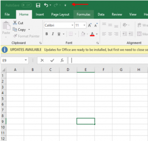
1. If you look at the top left of your toolbar, you will be able to see the small excel icons for autosave, undo and redo features. If you look right next to the “Redo” button, there is a drop-down button. This will take you to the next step.

       

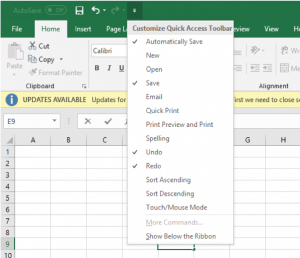
2. From here you can Customise Quick Access Toolbar, with features such as New, Open, Email, Quick Print, Print Preview and Print, Spelling, Sort Ascending, Sort Descending, Touch/Mouse Mode.
3. Add your chosen shortcuts to save you time on your next project.

Conditional Formatting

Conditional Formatting is a tool which enables you to highlight cells according to their value.

Here are two ways in which Conditional Formatting is helpful:

Highlighting Cells:

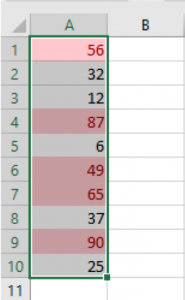
Highlighting cells gives you the ability to highlight cells depending on their value, including if they are greater than, or less than a certain number. If you have a larger amount of data, this can save you time when trying to highlight information.

1. Select the relevant range of cells
2. Click on “Conditional Formatting” on the toolbar
3. Click “Highlight Cell Rules”, then select “Greater Than”.

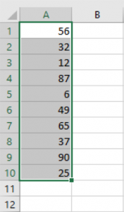
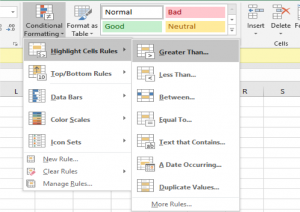
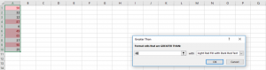
4. You can now enter the data you wish. We chose 48, so all cells with a higher value appear in red.

Clear Rules:

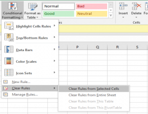
If you want to reverse the highlighted cells, here’s what you should do.

1. Select the relevant range of cells
2. Click on “Conditional Formatting” on the toolbar
3. Click “Clear Rules”, then “Clear Rules from Selected Cells”.

 

 

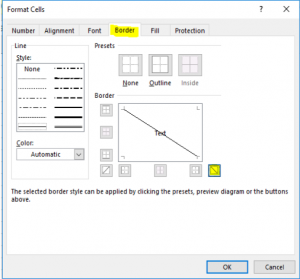
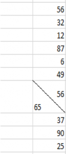
Add Diagonal Lines

Have you ever wondered how to add diagonal lines to your spreadsheets? Well here’s how you can.

This is a great way to separate data within a cell, making it easily presentable and simple to understand.

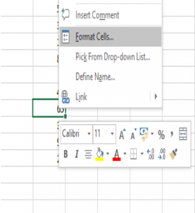
1. Select the cell you wish to add diagonal line to.
2. Click “Format Cells”.
3. Once you have the box, select “Border.”
4. Click the button to the bottom right of the text box.
5. To add text above and below the diagonal line, press Alt+Enter.
6. Use space bar to move the text to the opposite side of the cell.

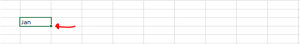
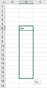
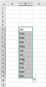
The Fill Handle

The fill handle automatically fills data dependent on the value or word you have entered. For this, we have chosen the word January, but it will fill out all the months of the year

1. Put in your word or value into the chosen cell
2. Drag the green box in the bottom of the cell, up or down.
3. Drag it to its chosen position
4. You should end up with automatically entered information.

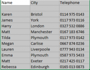
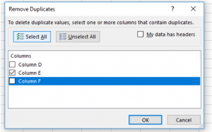
Remove Duplicates

 

It’s common when working with data that occasionally there may be duplicate information mistakenly entered onto the cells due to human error.

Excel can provide the answer and can remove all unwanted duplicate information at the click of a button.

1. First highlight the entire data set you wish to include.

1. Click “Data” tab.
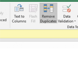
2. Click the “Remove Duplicates” button in the toolbar.
3. Select columns you want Excel to find duplicates in.
4. Hit “OK.”

Excel doesn’t always have to be difficult.

If you are looking to become more knowledgeable in Microsoft Excel, Elliott Training offer Excel Training Courses and other different IT courses from beginner to advanced level. We can help your business and your team bring these skills to life.

Want to book spaces on our courses or find out what’s on offer? Fill out a contact form or call us on 01454 203 355.